Plotting Manager Elo Ratings by Club Part 2

Recap

This is Part II of building a function to plot manager Elo ratings. If you haven’t yet, I recommend you read Part I first.

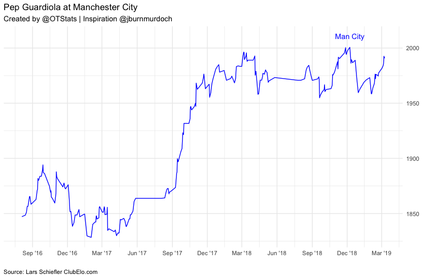
We left off with a graph of Manchester City’s Elo rating since Pep Guardiola has been manager.

Building a Function

In Part I I oversimplified a few steps, anticipating a few data discrepancies and glitches. I’ll do my best to identify the deliberate choices as they come up.

Disclaimer: There are definitely more efficient ways to accomplish our goal. I don’t claim to be an expert, and I’d love to hear recommendations on how to improve this process!

Step by Step

Recall the steps to achieve our goal:

1. Identify manager
2. Read data for each club managed
3. Filter each club’s Elo to manager’s era
4. Combine all clubs into one data frame
5. Select highest Elo by club for label
6. Plot data

We’ll start relatively simple by defining a function with an argument for a manager string. We’ll then refer to our packages and construct the url we’ll need for the API call. We’ll download the manager’s html file, and extract their club history.

  manager_club_history <- function(manager){
  needs(tidyverse, magrittr, scales, rvest, lubridate)
  
  # Prep for downloading manager data from manager's page on clubelo.com
  manager_url <- str_c("http://clubelo.com/", manager)
  manager_html <- str_c(manager, ".html")
  
  download.file(manager_url, dest = manager_html)
  raw <- read_html(manager_html) %>% 
    html_table(header = TRUE, fill = TRUE)
  
  manager_club_history <- raw[3][[1]]
  manager_club_history
  }

So far, our function will return a dataframe with a manager’s club history. Let’s see Arsene Wenger’s:

manager_club_history("ArseneWenger")
#     Club                From                  To      Days Games Elo ⌀ Elo points +/-
#1 Arsenal Mon, Sep 30th, 1996 Sat, Jun 30th, 2018 7944 days  1044  1850             60
#2  Monaco  Wed, Jul 1st, 1987 Thu, Jun 30th, 1994 2557 days   310  1686             31
#3   Nancy  Sun, Jul 1st, 1984 Tue, Jun 30th, 1987 1095 days   114  1454            -39

Now we need to write a sequence that will pull in the Elo history for each club. We can start by creating an empty dataframe, then looping through each row of manager_club_history to access: club name, from, and to. We’ll pull the club Elo history, filter to only dates within the manager’s tenure, then combine the rows to our dataframe manager_club_elo:

  # Set empty data frame
  manager_club_elo <- data.frame()
  # API call for each club
  for (i in 1:nrow(manager_club_history)){
    
    club_name <- manager_club_history[i, 1] %>% 
      str_remove_all(pattern = " ")
    
    base_url <- "http://api.clubelo.com/"
    club <- str_c(base_url, club_name)
    
    club_elo <- read_csv(club)
    
    start <- manager_club_history[i, 2] %>% 
      mdy()
    
    end <- manager_club_history[i, 3] %>% 
      mdy()
    end <- if_else(end > Sys.Date(), Sys.Date(), end)
    
    manager_single_club <- club_elo %>% 
      filter(From >= start & To <= end)
    manager_club_elo <- bind_rows(manager_club_elo, manager_single_club)
  }

From there, we’ll select the highest Elo by club for our labels:

  manager_club_labels <- manager_club_elo %>% 
    group_by(Club) %>% 
    top_n(1, Elo)

And lastly plot our data:

  manager_club_elo %>% 
    ggplot(aes(To, Elo, group = Club, color = Club)) + 
    theme_minimal() + 
    geom_line() + 
    geom_text(data = manager_club_labels, aes(y = Elo + 10, label = Club)) + 
    scale_color_discrete(guide = F) + 
    scale_y_continuous(position = "right") + 
    scale_x_date(date_breaks = "2 years", date_labels = "%Y") + 
    labs(title = manager_alias, 
         x = "", 
         y = "")

In total our combined script looks like this:

plot_manager_elo <- function(manager, manager_alias){
  needs(tidyverse, magrittr, scales, rvest, lubridate)
  
  # Prep for downloading manager data from manager's page on clubelo.com
  manager_url <- str_c("http://clubelo.com/", manager)
  manager_html <- str_c(manager, ".html")
  
  download.file(manager_url, dest = manager_html)
  raw <- read_html(manager_html) %>% 
    html_table(header = TRUE, fill = TRUE)
  
  manager_club_history <- raw[3][[1]]
  
  # Set empty data frame
  manager_club_elo <- data.frame()
  
  # API call for each club
  for (i in 1:nrow(manager_club_history)){
    
    club_name <- manager_club_history[i, 1] %>% 
      str_remove_all(pattern = " ")
    
    base_url <- "http://api.clubelo.com/"
    club <- str_c(base_url, club_name)
    
    club_elo <- read_csv(club)
    
    start <- manager_club_history[i, 2] %>% 
      mdy()
    
    end <- manager_club_history[i, 3] %>% 
      mdy()
    end <- if_else(end > Sys.Date(), Sys.Date(), end)
    
    manager_single_club <- club_elo %>% 
      filter(From >= start & To <= end)
    manager_club_elo <- bind_rows(manager_club_elo, manager_single_club)
  }

  manager_club_labels <- manager_club_elo %>% 
    group_by(Club) %>% 
    top_n(1, Elo)
  
  manager_club_elo %>% 
    ggplot(aes(To, Elo, group = Club, color = Club)) + 
    theme_minimal() + 
    geom_line() + 
    geom_text(data = manager_club_labels, aes(y = Elo + 10, label = Club)) + 
    scale_color_discrete(guide = F) + 
    scale_y_continuous(position = "right") + 
    scale_x_date(date_breaks = "2 years", date_labels = "%Y") + 
    labs(title = manager_alias, 
         subtitle = "Created by @OTStats | Inspiration @jburnmurdoch",
         x = "", 
         y = "", 
         caption = "Source: Lars Schiefler ClubElo.com") + 
    theme(plot.caption = element_text(hjust = 0))
}

Note: I did do a thing - I added an extra argument to our function manager_alias. This argument takes a character string, and is used in the title of my plot.

Explore Manager Elo’s

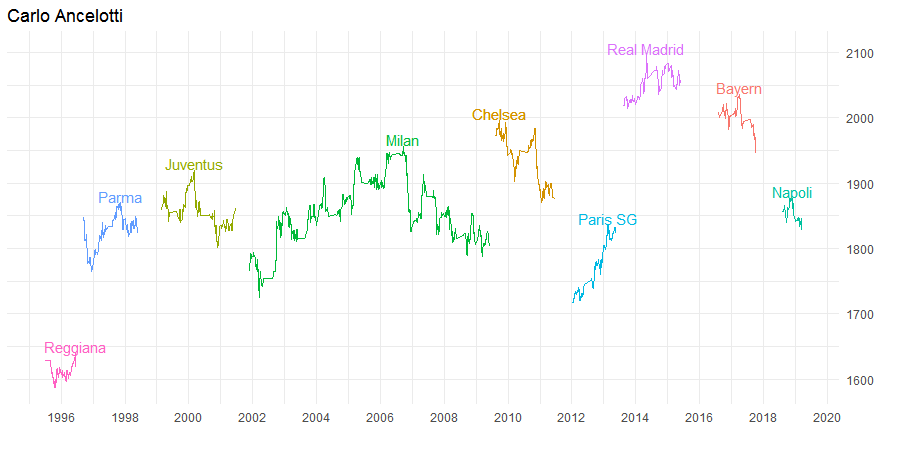
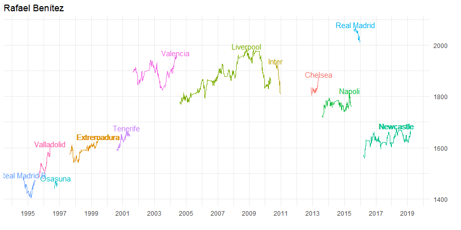
Now let’s look at a few famous managers!

Next Steps

Multiple stints with a club

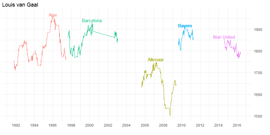
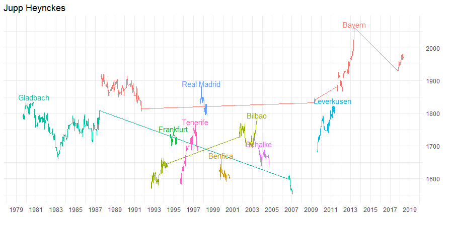
Did you notice anything weird on Jupp Heynckes and Louis van Gaal’s Elo history above?

• Louis van Gaal in between his two stints as manager of Barcelona, LvG took over as manager for the Dutch national team. This is important to note: ClubElo does not take into consideration international management.
• Jupp Heynckes, a historic manager in his own right, has managed the same club on multiple occasions… with three different clubs: Borussia Mönchengladbach, Athletic Bilbao, and Bayern Munich. If we want to get technical, Heynckes was Bayern’s manager on four separate occasions. After sacking Jürgen Klinsmann, he was appointed caretaker manager for 5 games.

So what happened to our graph? Recall that we passed the Club to the color aesthetic in our ggplot, R then assumes that these stints are related, which technically speaking is true, by Club. Let’s look at John’s code for Jose Mourinho, again.

...
jose.all <- bind_rows(
  jose.porto %>% filter(From >= as.Date("2002-01-22") & To <= as.Date("2004-06-30")),
  jose.chelsea %>% 
    filter(
      (From >= as.Date("2004-07-01") & To <= as.Date("2007-09-19"))
    ),
  jose.chelsea %>% 
    filter(
      (From >= as.Date("2013-07-01") & To <= as.Date("2015-12-17"))
    ) %>% mutate(Club = "Chelsea 2"),
  jose.inter %>% filter(From >= as.Date("2008-07-01") & To <= as.Date("2010-06-30")),
  jose.real %>% filter(From >= as.Date("2010-07-01") & To <= as.Date("2013-06-30")),
  jose.mufc %>% filter(From >= as.Date("2016-07-01") & To <= as.Date("2018-12-18"))
)
...

John made a very minor adjustment in his code - upon filtering Chelsea’s Elo history, he used mutate() to set Club to Chelsea 2. We’ll have to take this into consideration going forward.

Club names

When I was plotting managers’ Elo history I discovered that a few managers would return issues. Language became important. Take Unai Emery - current manager of Arsenal FC. Let’s read in Emery’s managerial history. Let’s make things simple use our manager_club_history function:

manager_club_history("UnaiEmery") %>% as.tibble()
## A tibble: 6 x 7
#  Club           From                To                  Days      Games `Elo ⌀` `Elo points +/-`
#  <chr>          <chr>               <chr>               <chr>     <int>   <int>            <int>
#1 Arsenal        Sun, Jul 1st, 2018  Sun, Jun 30th, 2019 231 days     39    1832               36
#2 Paris SG       Fri, Jul 1st, 2016  Sat, Jun 30th, 2018 730 days     92    1887              -17
#3 Sevilla        Mon, Jan 14th, 2013 Thu, Jun 30th, 2016 1264 days   182    1814               84
#4 Спартак Москва Sun, Jul 1st, 2012  Sun, Nov 25th, 2012 148 days     24    1693              -25
#5 Valencia       Tue, Jul 1st, 2008  Sat, Jun 30th, 2012 1461 days   196    1799               70
#6 Almería        Sat, Jul 1st, 2006  Mon, Jun 30th, 2008 731 days     80    1679              142

Ahh, we need to take into consideration special characters. We’ll have to consider logography, Cryllic script, and diacritic characters. This becomes an issue because we use Club to in our API call. Спартак Москва using the Latin alphabet is Spartak Moskva, or “Spartak Moscow”. The ClubElo url for the club is http://clubelo.com/SpartakMoskva, so when our loop tells R to retrieve data via the API there aren’t data to retrieve and our function stops with an error.

Better Aesthetics

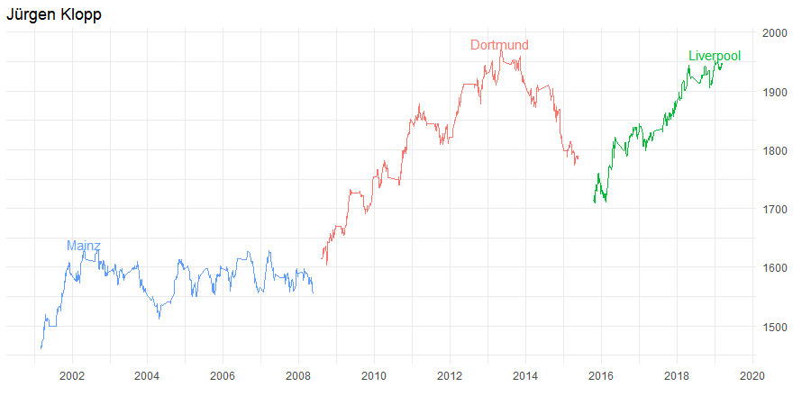
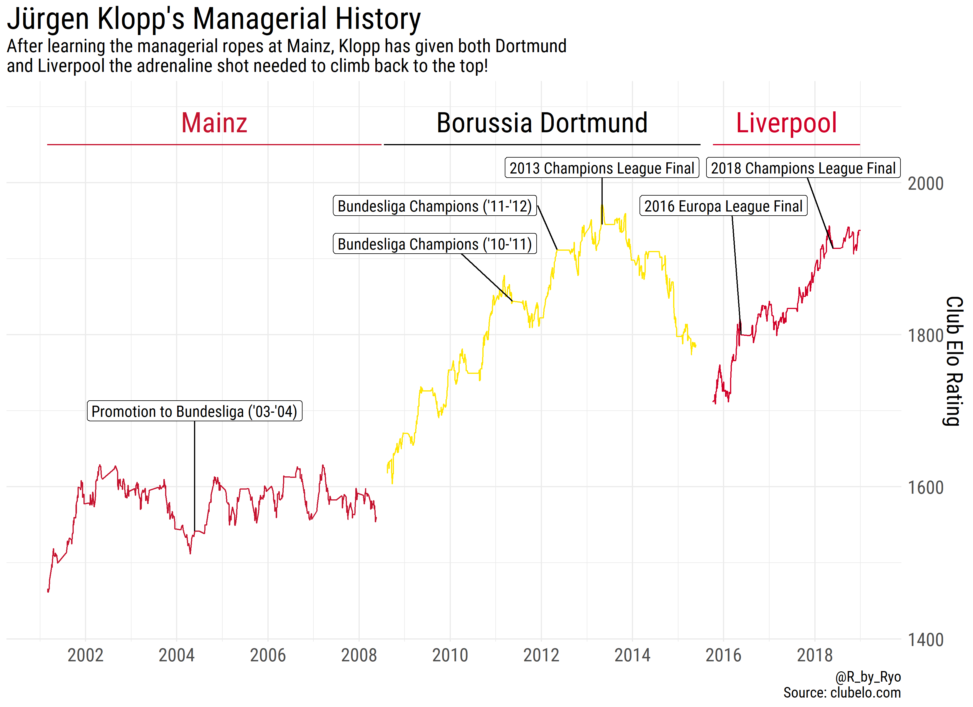
Thanks to the great R community on Twitter I stumbled across Ryo Nakagawara’s website, where he has published some beautiful data visualizations. He used a similar method as John to plot Juergen Klopp’s managerial history and also added a few extra aesthetic annotations. I’d love to add labels in a similar method that Ryo used at the top of his plot. I’d also love to define club colors in some fashion. Nothing against the ggplot’s default color palette but I can’t bear to see Real Madrid inherit green anymore.

End: Part II

That’s a wrap! I hope to revisit this script and data again in the future for some of my favorite managers.