Webscrape Disc Golf Stats

A few months into my (2020) quarantine one of my neighbors took me disc golfing. It wasn’t an entirely new experience for me, as I had gone a few times when I was younger, but this time around it really peaked my interest. In the days that followed I watched previous PDGA (Professional Disc Golf Association) events – catching a glimpse of how the discs are supposed to be thrown. The next week I bought a starter pack, and my fascination has since continued.

As I’ve gone on to watch a few of the professional disc golf events I’ve gotten familiar with some of the pros currently at the top of the game. Players such as Paul McBeth, Ricky Wysocki, Eagle McMahon, and Calvin Heimburg were regularly appearing in the final rounds of events of the men’s events, and Paige Pierce continuously dominated the women’s division. I began to wonder how much these professionals have earned across all these tournaments (although I’m sure some players also make a decent amount from their endorsements). Luckily the PDGA, the main governing body of professional disc golf, tracks most of this information. The PDGA website has a Player Statistics page that tracks annual earnings, ratings, and points for players of all PDGA-sanctioned events back to 1979. There didn’t appear to be any convenient way for me to compare these player’s earnings over time so I saw this as an opportunity to practice web scraping.

---

I started by scraping a single page to understand the structure of the web page (i.e. find the table within the HTML code). It took me about an hour to remind myself how to use inspect feature in Chrome to find the breadcrumb path to the HTML table, and I decided against including documentation about that process here (there are plenty of resources online about how that provide better documentation than I could).

#-- Load libraries
library(tidyverse)
library(polite)
library(rvest)
library(xml2)

# Read single page, rankings for 2019
url <- "https://www.pdga.com/players/stats?Year=2019&player_Class=All&Gender=All&Bracket=All&continent=All&Country=All&StateProv=All&page=0"

url %>% 
  bow() %>% 
    scrape() %>% 
    html_node("body") %>% 
    xml2::xml_find_first("//table") %>% 
    html_table() %>% 
    as_tibble()

## # A tibble: 20 x 12
##    Name  `PDGA #` Rating  Year Gender Class Division Country `State/Province` Events
##    <chr>    <int>  <int> <int> <chr>  <chr> <chr>    <chr>   <chr>             <int>
##  1 K. J…    41760   1037  2019 Male   Pro   Open     United… Arkansas             29
##  2 G. G…    13864   1030  2019 Male   Pro   Open     United… Florida              35
##  3 A. H…    68835   1027  2019 Male   Pro   Open     United… Oklahoma             32
##  4 C. H…    45971   1041  2019 Male   Pro   Open     United… Florida              30
##  5 P. M…    27523   1060  2019 Male   Pro   Open     United… California           23
##  6 J. C…    17295   1037  2019 Male   Pro   Open     United… Virginia             27
##  7 J. F…    69509   1029  2019 Male   Pro   Open     United… Colorado             32
##  8 S. L…     8332   1040  2019 Male   Pro   Open     United… Massachusetts        26
##  9 C. C…    50401   1026  2019 Male   Pro   Open     United… Missouri             27
## 10 A. P…    63765   1025  2019 Male   Pro   Open     United… Missouri             38
## 11 A. R…    66362   1028  2019 Male   Pro   Open     United… Washington           30
## 12 N. Q…    68286   1022  2019 Male   Pro   Open     United… North Carolina       40
## 13 E. O…    53565   1017  2019 Male   Pro   Open     United… Florida              25
## 14 R. W…    38008   1049  2019 Male   Pro   Open     United… South Carolina       22
## 15 E. M…    37817   1049  2019 Male   Pro   Open     United… Colorado             27
## 16 N. P…    65737   1021  2019 Male   Pro   Open     United… Texas                25
## 17 A. M…    75590   1021  2019 Male   Pro   Open     United… Michigan             34
## 18 A. H…    57365   1027  2019 Male   Pro   Open     United… Wisconsin            22
## 19 P. B…    26416   1022  2019 Male   Pro   Open     United… California           28
## 20 R. F…    48338   1013  2019 Male   Pro   Open     United… Michigan             33
## # … with 2 more variables: Points <int>, Cash <chr>

Voila. Now, a note about the actual URL string. The actual base URL for the PDGA Player Stats page is https://www.pdga.com/players/stats – much shorter than in the code snippet above. After playing around with a few of the filters on the page I found that they would also propagate in the URL. I also noticed there was an argument to filter year and page. So with some help from purrr, I could systematically pass a vector of years and a vector of page numbers to scrape PDGA player stats. First I can try scraping the top 100 players from 2019 – which would mean that I’d need to scrape pages 0 through 4 (as there are 20 players displayed per page). I can supply a base URL, clarifying Year=2019, and finish the URL string with page=, only to paste the base to a vector from 0 to 4, and map a predefined function to scrape the page as I just did.

base_2019 <- "https://www.pdga.com/players/stats?Year=2019&player_Class=All&Gender=All&Bracket=All&continent=All&Country=All&StateProv=All&order=Prize&sort=desc&page="

#-- Web scraping function
scrape_page <- function(url) {
  url_session = bow(url)
  url_session %>% 
    scrape() %>% 
    html_node("body") %>% 
    xml2::xml_find_first("//table") %>% 
    html_table() %>% 
    as_tibble()
}

(pdga_2019_top_100 <- str_c(base_2019, 0:4) %>% 
  map_df(~ scrape_page(url = .)))

## # A tibble: 100 x 12
##    Name  `PDGA #` Rating  Year Gender Class Division Country `State/Province` Events
##    <chr>    <int>  <int> <int> <chr>  <chr> <chr>    <chr>   <chr>             <int>
##  1 P. M…    27523   1060  2019 Male   Pro   Open     United… California           23
##  2 R. W…    38008   1049  2019 Male   Pro   Open     United… South Carolina       22
##  3 E. M…    37817   1049  2019 Male   Pro   Open     United… Colorado             27
##  4 J. C…    17295   1037  2019 Male   Pro   Open     United… Virginia             27
##  5 C. H…    45971   1041  2019 Male   Pro   Open     United… Florida              30
##  6 C. D…    62467   1041  2019 Male   Pro   Open     United… Tennessee            44
##  7 P. P…    29190    979  2019 Female Pro   Open Wo… United… Texas                26
##  8 G. G…    13864   1030  2019 Male   Pro   Open     United… Florida              35
##  9 K. J…    41760   1037  2019 Male   Pro   Open     United… Arkansas             29
## 10 C. A…    44184    977  2019 Female Pro   Open Wo… United… Minnesota            27
## # … with 90 more rows, and 2 more variables: Points <int>, Cash <chr>

---

Using the cross function from the purrr package, and a little code snippet in the function’s vignette, I was able to come up with an easy bit of code that did a lot. By running the next bit of code I accomplish the following:

1. define a function (same as above) to that will politely scrape the PDGA website and extract the HTML table and convert it to a tibble,
2. create a vector of all URL combinations for years 2015 through 2020 and pages 0 through 5 of the PDGA Player Stats page, and 3. passes that vector to map_df() with the aforementioned scrape_url (Note: this part of the script can take a little while, mainly because polite is using proper web scraping etiquette; my understanding is that it takes some time off between scraping pages).
3. The last little bits include some basic data cleaning (i.e. using janitor::clean_names() to clean up those variable names, and add a cash_value variable which converts the prize money from a character string to a numeric value).

Note: For a simple use case, I decided to use two predefined filters to select the men’s open division. I have future iterations in mind, which I’ll about later.

# -- Load libraries
library(tidyverse)
library(polite)
library(rvest)
library(xml2)
library(janitor)

# Define a function to scrape the PDGA player stats page and get the stats table
scrape_page <- function(url) {
  url_session = bow(url)
  url_session %>% 
    scrape() %>% 
    html_node("body") %>% 
    xml2::xml_find_first("//table") %>% 
    html_table() %>% 
    as_tibble()
}


# Source help (https://purrr.tidyverse.org/reference/cross.html)
pdga_params <- list(first_url_part = "https://www.pdga.com/players/stats?Year=", 
           years = 2015:2020, 
           second_url_part = "&player_Class=1&Gender=Male&Bracket=MPO&continent=All&Country=All&StateProv=All&order=Prize&sort=desc&page=", 
           pages = 0:4)

pdga_raw_scrape <- pdga_params %>% 
  cross() %>% 
  map(lift(paste0)) %>% 
  unlist() %>% 
  map_df(~ scrape_page(url = .)) %>% 
  janitor::clean_names() %>% 
  mutate(cash_value = str_remove_all(cash, "\\$|,") %>% as.numeric())

glimpse(pdga_raw_scrape)

## Rows: 600
## Columns: 13
## $ name           <chr> "P. McBeth", "R. Wysocki", "W. Schusterick", "N. Locastro",…
## $ pdga_number    <int> 27523, 38008, 29064, 11534, 12626, 27171, 8332, 11794, 3370…
## $ rating         <int> 1053, 1043, 1027, 1036, 1030, 1021, 1026, 1032, 1022, 1027,…
## $ year           <int> 2015, 2015, 2015, 2015, 2015, 2015, 2015, 2015, 2015, 2015,…
## $ gender         <chr> "Male", "Male", "Male", "Male", "Male", "Male", "Male", "Ma…
## $ class          <chr> "Pro", "Pro", "Pro", "Pro", "Pro", "Pro", "Pro", "Pro", "Pr…
## $ division       <chr> "Open", "Open", "Open", "Open", "Open", "Open", "Open", "Op…
## $ country        <chr> "United States", "United States", "United States", "United …
## $ state_province <chr> "California", "South Carolina", "Georgia", "Missouri", "Geo…
## $ events         <int> 26, 24, 30, 33, 30, 42, 26, 19, 29, 23, 28, 19, 29, 23, 19,…
## $ points         <int> 22100, 20822, 20115, 20895, 21092, 22867, 16557, 17487, 186…
## $ cash           <chr> "$72,044.70", "$34,565.00", "$32,633.00", "$27,519.00", "$2…
## $ cash_value     <dbl> 72044.70, 34565.00, 32633.00, 27519.00, 25876.39, 24284.00,…

At this point we can start asking and answering question with our data. For example, what players made the most money from PDGA sanctioned events from 2015 to 2020?

pdga_raw_scrape %>% 
  group_by(name) %>% 
  summarize(total_cash = sum(cash_value)) %>% 
  arrange(desc(total_cash)) %>% 
  mutate_at("total_cash", scales::dollar_format()) %>% 
  head(10) %>% 
  knitr::kable("pipe")

name	total_cash
P. McBeth	$333,390
R. Wysocki	$292,219
C. Dickerson	$177,685
E. McMahon	$167,060
P. Ulibarri	$140,892
N. Locastro	$135,026
S. Lizotte	$125,499
J. Koling	$121,203
J. Conrad	$119,402
N. Sexton	$117,217

Or we can look at annual earnings for the players that have won the most money between 2015 and 2020:

pdga_raw_scrape %>% 
  inner_join(pdga_raw_scrape %>% 
               group_by(name) %>% 
               summarize(total_cash_value = sum(cash_value)) %>% 
               arrange(desc(total_cash_value)) %>% 
               mutate(total_cash = total_cash_value %>% scales::dollar()) %>% 
               head(9) %>% 
               mutate_at("name", factor)) %>% 
  group_by(name = str_c(name, " - ", total_cash)) %>% 
  ggplot(aes(x = year, y = cash_value)) + 
  geom_col(fill = "#457b9d") + 
  scale_x_continuous(breaks = 2015:2020) + 
  scale_y_continuous(breaks = c(0, 25000, 50000, 75000), labels = scales::dollar_format())+ 
  expand_limits(y = 0) + 
  facet_wrap(~fct_reorder(name, total_cash_value, .desc = T)) + 
  theme_minimal() + 
  labs(title = "Paul McBeth and Ricky Wysocki win a lot", 
       subtitle = "Annual winnings of the top 9 men's players with the highest earnings from the PDGA-sanctioned\nevents between 2015 and 2020. Total earnings between 2015 and 2020 next to players name.", 
       x = "", 
       y = "", 
       caption = "Created by @OTStats\nData from PDGA.com") + 
  theme(plot.title = element_text(size = 20), 
        plot.subtitle = element_text(size = 10), 
        plot.caption = element_text(color = "#6c757d"), 
        axis.text.x = element_text(size = 8))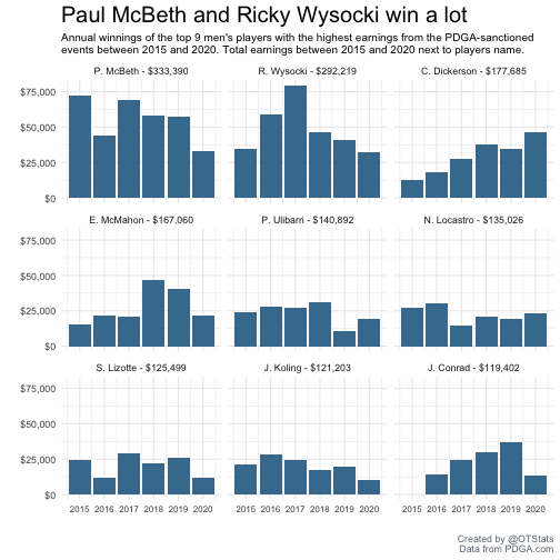

---

Future iterations

I see a ton of possibilities to expand on after this exercise. The obvious would be to expand the data set to include all other divisions. I also started working on a systematic way to visit player stats from a given year, identify the total number of players for the respective year from the HTML footer at the bottom of the page, and cycle through all available pages (e.g. there were +18K player records available in 2019, which would equate to over 900 pages). The program would take a bit of time to run, but it’d be a one-and-done process to get historical data, but I could add new years after the tournament season is over. I’d also love to dive into some of the stats available on individual player pages. These provide details of tournaments that players took part (such as the date, where they finished, and how much they made). I haven’t explored the player rating system, but it’s something I’ll probably explore later. Once I have a decent data set, my goal is to create an R package to house all of this data and publish to CRAN. This is hopefully something I can accomplish by the end of this year!